What is a battlecruiser?
An example of no-code machine learning

One thing that I’ve found mildly puzzling for a long time is the question of what exactly it means for a ship to be a “battlecruiser.” This is partly a historical issue, but on a certain level, it’s about trying to find a coherent and consistent definition for a label that wasn’t used consistently and coherently.

In this article, I’ll present a highly sophisticated and robust machine learning approach to defining a battlecruiser … using Google Sheets instead of R, Python, or C#. After training an ensemble classifier on a set of ships that nobody disputes are battlecruisers, I will seek to answer the following questions:
Is “battlecruiser” a single coherent category?
Which post-WWI ships were battlecruisers in all but name?
Is a battlecruiser more like a cruiser - or more like a battleship?
The spreadsheet is here. I’ll walk through how a Bayesian pack works - an ensemble of Bayesian classifiers.
A little background
In 1905, the Japanese defeated the Russians in the Battle of Tsushima. At the time, there were two types of capital ships, today known as pre-dreadnought battleships and armored cruisers. These ships were similar in size and cost; battleships generally had more armor and firepower, while armored cruisers were faster. The Japanese fleet was led by four pre-dreadnought battleships and eight armored cruisers; the Russian fleet was led by eight pre-dreadnought battleships and two armored cruisers.

The Japanese ran circles around the Russians with superior speed, rate of fire, accuracy, and communications. In response to that battle, the British designed the HMS Dreadnought, a revolutionary new ship that had the speed of an armored cruiser, the armor of a battleship, and firepower comparable to two battleships. This development was spearheaded by First Sea Lord Jackie Fisher.

Fisher’s blazingly fast new battleship was revolutionary enough to set off an immediate arms race, but he wasn’t done. Working by the maxim “speed is armor,” he came up with an even more revolutionary successor to the armored cruiser: The battlecruiser. The armored cruiser sacrificed both firepower and armor in order to gain speed over its battleship counterparts; the battlecruiser would mainly sacrifice armor, with firepower comparable to the new dreadnoughts. A battlecruiser would be able to threaten any other ship with destruction and successfully disengage from any ship that could threaten it with destruction.
The Germans, neck-deep in a naval arms race with the British, responded by building their own battlecruisers. The German battlecruiser was designed to try to outfight anything that it couldn’t outrun, and outrun anything it couldn’t fight. Like an armored cruiser, it balanced armor and firepower while prioritizing speed. From the very beginning, battlecruiser as a category included two strikingly different design philosophies. Then came World War I.
For various political and economic reasons, World War I halted the naval arms race in its tracks and major powers stopped building dreadnoughts and battlecruisers for a little while. The USS West Virginia, laid down in 1920, is clearly a dreadnought. The USS Lexington, laid down in 1921, was clearly designed to be a battlecruiser. When the US Navy ordered its next round of capital ships in 1937, there were no separate battlecruisers and dreadnoughts, only the North Carolina class battleships … which were faster than any pre-Jutland dreadnought and better armored than any pre-Jutland dreadnought.
The naive Bayesian classifier
There are a lot of different ways to create machine learning classifiers. One of the more theoretically straightforward ways to try to figure out how to classify different objects into categories is to use statistics on quantifiable measurements.
The naive Bayesian classifier uses Bayes’s theorem to calculate the probability that an object belongs to a given category.
Here, P(B|X) is the probability that B is true given X is true. If each category out of the list of possible categories is equally likely, this simplifies to:
That is to say, the probability that an object belongs to a given category is equal to the sum of all the probability density measurements at that point. The nice thing about this is that probability density functions are usually easy to estimate. Thus, if we have two categories, A and B, and they’re distributed as in the plot below, a measurement of x=2.3 corresponds to a probability density of p = 0.8 for category A and p = 0.08 for category B, meaning there’s about 10-out-of-11 (91%) chance that the object belongs to category A.

Similarly, if x = 3.0, then the ratio of the density functions is (0.05/(0.22+0.05)), which means that there’s only about a 19% chance the object belongs to category A. This is a statistically sound method of calculating probabilities, and “naive” means we’re going to ignore something, so what are we ignoring? Well, here are the “naive” assumptions we’re making:
The variables we’re measuring are normally distributed, that is to say, their probability density functions look like a bell curve.
The variables we’re measuring are independent, which is to say, they’re not inherently related to each other.
The categories are equally likely to apply to whatever object we’re trying to classify.
These assumptions are rarely true in the real world, but they’re usually approximately true if we take some care with choosing what we measure. Height and weight, for example, are closely correlated (taller people are usually also heavier), but height and BMI are much more weakly related.1
Choosing measurements
I’ve chosen seven raw measurements to rely on. They are not at all independent, but they’re easy to obtain. These raw measurements (along with the year the ship was laid down) are entered in the “Data entry” sheet of the spreadsheet.
Maximum displacement (mass), measured in metric tons
Maximum speed, measured in knots
Engine power, measured in horsepower
Caliber (size) of largest guns, measured in millimeters
Mass of a single salvo from the main battery, measured in kilograms2
Belt armor
Turret armor
Size is a variable that can’t be successfully used to distinguish between battlecruisers and dreadnoughts; instead, it mostly varies with the age of the capital ships, with capital ships of all kinds growing larger over time. However, size can be used to decorrelate the other measurements.
For salvo mass and engine power, I’ll divide by displacement. For belt armor thickness and caliber, I’ll divide by the cube root of displacement. For turret armor, I’ll divide by gun caliber. This gives us two size-neutral and mostly uncorrelated variables related to maneuverability, durability, and offensive firepower. If we combine each pair of variables, this gives us three general variables that cover maneuverability, durability, and firepower.3 Each of those three measures should be independent.

These variables go in the “Transformed variables” sheet. I could have just put them in the same sheet, but this makes it easier to make sure manual data entry is confined to a single human-readable sheet in the spreadsheet.
Exploratory analysis
Even if we think we’ve gotten ourselves three nicely independent variables, we should explore a little bit about what’s going on with the variables. If you’re following along in the spreadsheet, click on “Exploratory table” for a minute. This is what’s known as a pivot table, generated by Insert => Pivot Table => In New Sheet. There are a couple of key issues to highlight here.

First, there are some pretty major differences between battlecruisers built by the British before Jutland and battlecruisers built or designed by the Germans. This most notably included a difference in armor; Admiral Jackie Fisher went by the maxim that speed was armor, and British battlecruisers were underarmored. Japanese, Russian, and American battlecruisers followed suit.4
Second, dreadnoughts don’t just get bigger over time; they get a little faster, a little better armored, and much more powerful in the later generation (known as superdreadnoughts). What this means is that when we try to figure out whether or not later battleships look like battlecruisers in all but name, we’ll use two classifiers:
One simply looks at all dreadnoughts and all battlecruisers as two groups.
The other uses three groups: Superdreadnoughts, German battlecruisers, and British battlecruisers.
These different approaches will give slightly different answers.
Training and using classifiers
To “train” a naive Bayesian classifier is as simple as calculating the mean and standard deviation of your training sample for each of the variables in mind. This is done in the sheets titled “Average 1,” “Average 2,” “SD 1”, and “SD 2,” which are also pivot tables.
These probability distributions are then applied to each ship in the data set in the “_scores” sheets, starting with “AC_scores” (armored cruiser scores). These sheets calculate the probability density of the inferred distribution. Then these scores are transformed into multivariate probability density scores in the “_p” sheets, starting with “AC_p.”

Each of the classifiers uses a product of three variables, one linked to maneuverability, one linked to durability, and one linked to firepower. The nine different classifiers in the sheet use nine different combinations of variables. So, for example, Classifier #5 uses engine power, turret armor, and broadside weight. On this basis, the famous USS Maine looks a lot more like a typical armored cruiser than the HMS Hood. Note this score isn’t a probability - in the above example, the probability density is actually greater than 1!
To get a probability, we have to sum over all possibilities. So, for example, in the case of the Maine, designated as ACR-1, we know by virtue of its age and some of the design features that aren’t in the spreadsheet, it’s either an armored cruiser or whether it was a pre-dreadnought battleship.5

In this case, Classifier #5 estimates there’s a 16% chance the Maine is an armored cruiser. Most of the other classifiers are more pessimistic. If we average over all nine classifiers, the group of classifiers - called an ensemble - estimates that the USS Maine looks 95% like a battleship rather than an armored cruiser. In fact, if we include all of our training categories, the Maine still looks a lot like a pre-dreadnought battleship (87% classifier score).
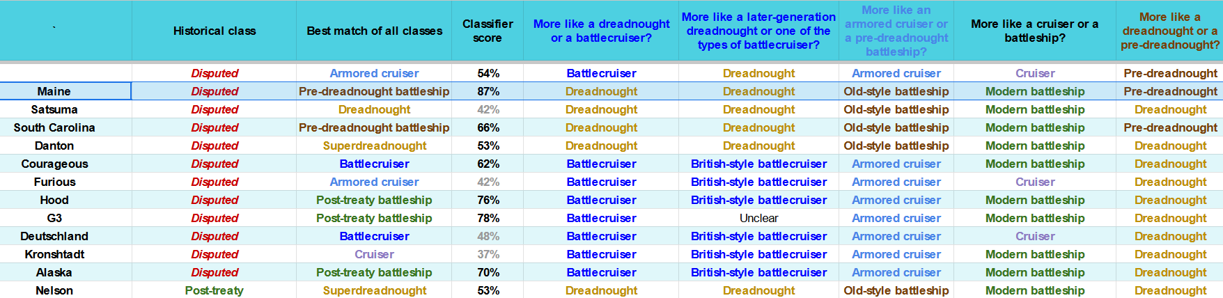
Applying this method to other ships of disputed status tells us that out of the early “semi-dreadnoughts” Satsuma, South Carolina, and Danton, the South Carolina really doesn’t look like a dreadnought - more like a late pre-dreadnought. The Hood (and the canceled G3 battlecruiser) really look like post-treaty fast battleships.
While they may have been small, the Deutschland class “pocket battleships” really look a lot more like battlecruisers than cruisers. On the other end of the scale, the Alaska class, billed as a “large cruiser,” looks a lot more like a battleship or battlecruiser than a mere oversized cruiser. In fact, in spite of its relatively thin armor, it looks more like a modern battleship than any particular sort of battlecruiser.
Where did the battlecruisers go?
While the British had no qualms about classifying HMS Hood as a battlecruiser in 1920, later naval historians have had doubts. However, the fundamental distinction between battlecruisers and dreadnoughts was in their balance of speed, firepower, and armor. Even if we don’t consider the Hood, most post-treaty battleships look more like battlecruisers than dreadnoughts.

The fact of the matter is that the balance between speed, armor, and firepower of the most fast battleships looks closer to the balance of speed, armor, and firepower that was used on German battlecruisers. Relative to their size, later battleships had smaller guns than slow dreadnoughts, and an enormously larger investment in speed.
The two biggest exceptions are the Nelson class (which was essentially one last late superdreadnought) and the Yamato, which made such an enormous investment in armor thickness and guns that it looks more like a dreadnought than a battlecruiser.

On average, the post-treaty battleships simply look more like battlecruisers than dreadnoughts, and in most cases most like German-style battlecruisers or the HMS Hood. At best, post-treaty battleships as a group split the difference between dreadnoughts and battlecruisers.
Re-evaluating the “dead end” of battlecruisers
From the machine learning model, we can gain some quantitative insight into a historical question: What exactly was a battlecruiser? It’s not uncommon for buffs of naval history to say that battlecruisers were a type of cruiser, or that armored cruisers were a dead end in warship development.
Jackie Fisher’s treasured HMS Dreadnought wasn’t a pure descendant of pre-dreadnought battleships. It is better considered a hybrid of the armored cruisers Fisher admired with the battleships the rest of the Admiralty preferred. Similarly, battlecruisers were not an offshoot of dreadnoughts; Jackie Fisher had the first of both types of ship designed at the same time. More than anything else, battlecruisers were designed to be the purest refinement of existing armored cruisers into a more effective form.
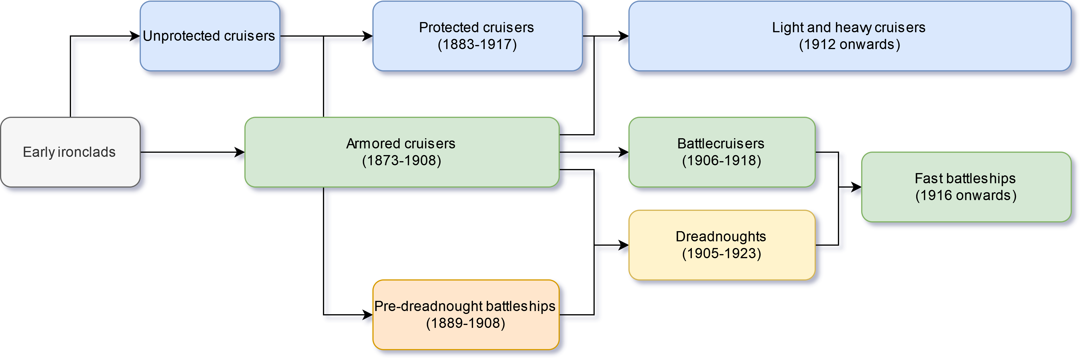
At the very beginning, “armored cruiser” simply meant a ship capable of operating effectively on independent long range missions that also had belt armor, as distinct from a coastal battleship. Many of the very earliest armored cruisers, such as the Maine, more closely resemble pre-dreadnought battleships than later armored cruisers.
While similar to dreadnoughts in some ways, fast battleships were more similar to battlecruisers, particularly the German battlecruisers, which had a better balance of armor and firepower. At the least, fast battleships were an even cross between battlecruisers and dreadnoughts. Given that dreadnoughts were roughly even cross between pre-dreadnoughts and armored cruisers, it’s not surprising that fast battleships register as being more closely akin to armored cruisers than to pre-dreadnought battleships by a large margin.
Interestingly, some of the ships “misidentified” by the classifier point toward a general trend of dreadnoughts evolving to become more like battlecruisers; the Japanese Nagato class, one of the very last dreadnought classes built before the Washington Naval Treaty paused new construction, registers as being like a German battlecruiser. So does the never-built Francesco Caracciolo class that was canceled by the onset of World War One. Both of these classes are frequently described as having been fast battleships.
BMI divides weight by the square of height. This works approximately if you’re only dealing with adults in a normal height range. To properly decorrelate weight with height more precisely, something closer to height cubed is required - IME, the 2.5th power is generally sufficient.
Since having a uniform main battery is one of the revolutionary characteristics of dreadnoughts and battlecruisers, pre-dreadnoughts and armored cruisers have their “main battery salvo” calculated including their broadside weapons down to as small as 6”.
To combine them, I normalized both variables in each pair before summing together, so that each variable has roughly the same impact on the combined measure.
The British built the first Japanese battlecruiser and advised the Russians in the construction of their battlecruisers. The American Lexington class, eventually converted to aircraft carriers, was designed with the Japanese Kongo and British Admiral classes in mind. French battlecruiser design studies were most similar to later German designs.
Both terms were used to refer to the Maine in contemporary sources, even if the designation “ACR-1” made it officially an armored cruiser.